Deep Learning for Developers: Tools You Can Use to Code Neural Networks on Day 1

Deep learning is one of the most exciting and powerful fields in technology today. At a high level, deep learning refers to using artificial neural networks to automatically learn patterns and extract insights from data – whether images, text, audio, videos, sensor readings, or other complex, high-dimensional data.

By discovering intricate structures in large datasets, deep learning has achieved state-of-the-art results and sometimes superhuman performance on a variety of tasks – recognizing objects in images, understanding natural language, making recommendations, diagnosing diseases, discovering new drugs, and controlling robots, to name just a few. Companies like Google, Facebook, and Apple are making huge investments in deep learning to power new features and products.

So what exactly is a neural network? At its core, a neural network is a complex mathematical function with millions of parameters that can map raw inputs to useful outputs. The network is composed of layers of artificial "neurons" that are connected with weighted edges. Each neuron computes a simple function of its inputs and passes the output to neurons in the next layer. By composing together dozens or hundreds of these layers, the network can learn very complex, non-linear relationships in the data.

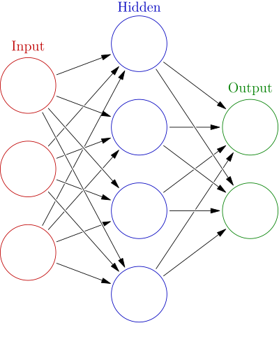
^{Diagram of a simple feedforward neural network. Source: Wikipedia}

Training a neural network involves showing it millions of labeled examples and gradually adjusting the connection weights to minimize a loss function that measures the difference between the network‘s predictions and the true labels. This optimization process, called gradient descent, is guided by the gradient of the loss function with respect to each weight, which can be efficiently computed using the backpropagation algorithm. By iteratively updating the weights to follow the negative gradient, the network eventually converges to a state that can accurately map inputs to the correct outputs.

While the mathematical details can get complex, the good news is that you don‘t need to derive the equations yourself or implement everything from scratch in order to start using neural networks. In the past few years, several powerful open source frameworks have emerged that provide high-level abstractions for defining and training neural networks, making it simpler than ever to get started with deep learning.

Popular Deep Learning Frameworks

Some of the most popular deep learning frameworks used in industry and academia include:

TensorFlow – Developed by Google, TensorFlow is a powerful library for dataflow programming and has built-in support for deep learning. Models are defined as directed graphs of mathematical operations that efficiently map data through multiple GPU or CPU devices. TensorFlow has a large ecosystem of extensions and supported models.

Keras – Keras is a high-level API written in Python that makes it easy to define, train and evaluate neural networks. It can use TensorFlow, CNTK or Theano as its backend to handle the low-level computations. Keras has a simple, intuitive interface and is designed for fast experimentation.

PyTorch – PyTorch is an open-source library for deep learning developed by Facebook. It has an imperative style that makes debugging easier, and supports dynamic computation graphs that can be defined on the fly. PyTorch is known for being clean and easy to use.

Caffe – Caffe is another deep learning framework, originally built by Berkeley AI researchers, that is known for its speed and efficiency. It has a large repository of pre-trained models for image classification, segmentation and more.

MXNet – Developed by Apache, MXNet is a lean, flexible framework that allows you to define, train and deploy neural networks on a wide range of devices from CPUs to mobile phones to distributed GPU clusters. It has a concise API and claims to have excellent performance and scalability.

These are just a few of the many deep learning frameworks out there (others include CNTK, Chainer, Theano, DeepLearning4J and more). They share many common concepts but differ in the details of their architecture and implementation. Ultimately, the best framework to use depends on your preferences, needs and existing software stack.

For this post, we‘ll focus on Keras since it has a beginner-friendly API, but the concepts apply to any framework. Let‘s dive into a code example of using Keras to build a neural network for a toy problem.

Implementing a Neural Network in Keras

We‘ll tackle the classic "Hello World" of machine learning – the MNIST handwritten digit classification dataset. This dataset contains 60,000 grayscale images of digits from 0 to 9 that were hand-drawn by high school students and employees of the US Census Bureau. Each image is 28×28 pixels. The goal is to train a neural network that can accurately classify new images of handwritten digits.

First, let‘s load the MNIST dataset using some convenient utilities in Keras:

from keras.datasets import mnist

(train_images, train_labels), (test_images, test_labels) = mnist.load_data()

This loads the dataset from a local cache or downloads it if needed, giving us 60,000 labeled training images and 10,000 test images stored as multi-dimensional Numpy arrays.

Next, we need to preprocess the data by reshaping the images into flat vectors and normalizing the pixel intensities to be between 0 and 1:

train_images = train_images.reshape((60000, 28 * 28))
train_images = train_images.astype(‘float32‘) / 255

test_images = test_images.reshape((10000, 28 * 28))
test_images = test_images.astype(‘float32‘) / 255

We‘re now ready to define our neural network model. We‘ll use a simple feedforward network (also called a multilayer perceptron) with two fully-connected hidden layers. The input layer has 784 units corresponding to the flattened pixels of the 28×28 images. The hidden layers have 512 units each and use the ReLU activation function. The final output layer has 10 units corresponding to the 10 digit classes, and uses the softmax activation to output a probability distribution over the classes.

Here‘s how we define this model in a few lines of Keras code:

from keras.models import Sequential
from keras.layers import Dense

model = Sequential()
model.add(Dense(512, activation=‘relu‘, input_shape=(28 * 28,)))
model.add(Dense(512, activation=‘relu‘)) 
model.add(Dense(10, activation=‘softmax‘))

The Sequential model is a linear stack of layers where the output of each layer is the input to the next. We use the add() method to add Dense fully-connected layers one after the other. The first layer needs to specify the shape of its input, which matches the size of our flattened MNIST images.

We can inspect the architecture of our model by calling the summary() method:

model.summary()

This displays:

_________________________________________________________________
Layer (type)                 Output Shape              Param #   
=================================================================
dense_1 (Dense)              (None, 512)               401920    
_________________________________________________________________
dense_2 (Dense)              (None, 512)               262656    
_________________________________________________________________
dense_3 (Dense)              (None, 10)                5130      
=================================================================
Total params: 669,706
Trainable params: 669,706
Non-trainable params: 0
_________________________________________________________________

Our network has a total of 669,706 learnable parameters – these are the weights and biases of the connections between neurons that will be tuned during training to minimize the loss.

To train the network, we first need to configure the learning process by specifying an optimizer, a loss function, and some metrics to monitor:

model.compile(optimizer=‘rmsprop‘,
              loss=‘categorical_crossentropy‘,
              metrics=[‘accuracy‘])

Here we‘re using the efficient RMSProp optimizer with a learning rate of 0.001, and the cross-entropy loss which is appropriate for multi-class classification. We‘ll keep track of the accuracy metric while training.

Finally, we can kick off the training process by calling the fit() method:

model.fit(train_images, train_labels, epochs=5, batch_size=128)

This trains the model for 5 epochs (complete passes through the training set) using mini-batches of 128 images at a time. On my machine, each epoch takes about 5 seconds, and we reach a final validation accuracy of about 98%! Not bad for a few lines of code.

Once the model is trained, we can evaluate its performance on the test set:

test_loss, test_acc = model.evaluate(test_images, test_labels)
print(‘Test accuracy:‘, test_acc)

The model achieves about 97.8% accuracy on the held-out test images – it can correctly classify handwritten digits that it has never seen before!

We can also use the trained model to make predictions on new images:

predictions = model.predict(test_images[:5])
print(predictions)

This outputs a 5×10 matrix where each row contains the predicted probabilities of the 5 test images belonging to each digit class.

That covers the basics of defining, training, and evaluating a neural network in Keras. We can make the model more powerful by adding more layers, increasing the number of units, using different activation functions and regularization techniques, or tuning the training settings – but this gives you a sense of how quickly you can get a working baseline with deep learning.

Scaling Up with Cloud GPUs

While our simple MNIST model can be trained on a laptop CPU in a reasonable amount of time, most real-world deep learning models are far more complex and have millions or billions of parameters. Training them requires an enormous amount of computation, often taking days or weeks on powerful hardware.

Fortunately, deep learning frameworks like TensorFlow and PyTorch can take advantage of GPUs (graphics processing units) to accelerate the math-heavy operations used in training neural networks. A single GPU can provide a 10-50x speedup over a fast multi-core CPU.

To speed up training even further, we can use multiple GPUs in parallel, either on the same machine or across a distributed cluster. TensorFlow and PyTorch make it easy to scale training with very little code changes.

While building your own deep learning rig is certainly a fun engineering challenge, a more practical and cost-effective option for most people is to rent GPU instances from a cloud provider like AWS, Google Cloud, or Azure and run your models there. With a few clicks or CLI commands, you can spin up an instance pre-configured with CUDA drivers, deep learning frameworks, and all the dependencies you need to start training models at scale.

If you‘re using Keras, you can start with one of the many code examples and run it on a cloud GPU with very little modification. I‘d recommend checking out Floyd, which provides an easy-to-use platform for running deep learning jobs in the cloud. It has a Heroku-like workflow where you can launch a TensorFlow or PyTorch environment, upload your code via Git or web IDE, and kick off model training and evaluation with a simple CLI.

Deep Learning Best Practices

Debugging a misbehaving neural net can sometimes feel like more art than science, but here are some general tips and tricks I‘ve found useful for building better models:

Start simple – Begin with a small network and get the end-to-end training loop working before adding more layers. Don‘t be afraid to experiment.

Visualize everything – Plot metrics like loss, accuracy, activations, and gradients. Visualizing the model‘s performance over time and on individual examples can provide valuable clues for debugging.

Use the right loss function – Make sure you‘re using an appropriate loss that measures what you care about. For example, use cross-entropy loss for classification, mean squared error for regression.

Normalize your inputs – Subtract the mean and divide by the standard deviation of each feature so that they have zero mean and unit variance. This helps the optimization converge faster.

Initialize weights carefully – The initial weights can have a big impact on the model‘s ability to learn. Use techniques like Xavier/Glorot or He initialization to set sensible starting values that avoid vanishing or exploding activations.

Use a good optimizer – Adam, Adadelta, and RMSProp are usually safe bets that perform well across many problems. SGD with Nesterov momentum or learning rate annealing can also work well.

Monitor training dynamics – Keep an eye on ratios like update size / parameter scale, or gradient norm / parameter norm, which measure the stability of the training process. Values above 0.01 indicate unstable updates.

Regularize – Applying L1 or L2 regularization to the weights, or using dropout (randomly zeroing out a fraction of activations), can prevent overfitting by making the model more robust to noise.

Hyperparameter search – Automatically tune the model‘s hyperparameters using techniques like grid search, random search, or Bayesian optimization to find the optimal settings for learning rate, batch size, etc.

What‘s Next?

This post has only scratched the surface of what‘s possible with deep learning. Once you‘ve got the basics down, here are some more advanced topics and applications to explore:

• Convolutional neural networks for computer vision
• Recurrent neural networks for sequence modeling
• Unsupervised learning with autoencoders and GANs
• Reinforcement learning for control and game-playing
• Transfer learning for adapting pre-trained models to new tasks
• Multimodal learning for jointly reasoning over text, images, audio, etc.
• Deploying models to production for inference and serving predictions

I‘d encourage you to dive into the references below and start experimenting with building your own neural networks. Deep learning is a powerful tool to have in your developer toolkit, and the barriers to entry are lower than ever thanks to the amazing open-source frameworks and tools now available. What will you create?

References and Further Reading

• Deep Learning Book – Comprehensive textbook on the theory and practice of deep learning.
• Deep Learning Specialization – Online courses on neural networks, CNNs, RNNs, and more, taught by Andrew Ng.
• Fast.ai – Practical deep learning courses for coders focused on real-world applications.
• Keras Documentation – User guides and code examples for the Keras deep learning library.
• CS231n Convolutional Neural Networks for Visual Recognition – Thorough treatment of the fundamentals of neural networks and CNNs by Andrej Karpathy and colleagues.